

Graph Signal Processing: A Short History, and Who Is Building It
Published:
Classical signal processing assumes a regular domain. A time series is indexed by a line, an image by a grid, and everything downstream — the Fourier transform, filtering, sampling, convolution — inherits the regularity of that index set. Shift a signal one sample to the right and it is still the same signal, moved. That single property is what the whole edifice is built on.
Most of the data I work with has no such domain. Cells sit in tissue at irregular positions. Brain regions connect through a structural network. Genes relate through co-expression. There is no “one sample to the right.” The index set is a graph, and the question graph signal processing (GSP) asks is deceptively simple: if the domain is a graph rather than a line, what does frequency mean?
This is a history of how that question got asked, answered twice, and carried into biology — with a list of the people whose work the field currently rests on.
Every figure below is computed, not drawn: the eigenvectors are the actual Laplacian eigenvectors of the graph beneath them, and the spectra are the actual graph Fourier coefficients of the signals shown. The script that produces them is in the site repository.
Prehistory: spectral graph theory (1973–2011)
The mathematics arrived long before the signal-processing framing.
The central object is the graph Laplacian, L = D − A, where A is the adjacency matrix and D the diagonal degree matrix. Its quadratic form is
which is exactly the total disagreement between neighbours. A signal that varies little across edges has a small value; one that flips sign at every edge has a large one. So L measures roughness — and its eigenvectors, ordered by eigenvalue, are ordered from smoothest to roughest. That is the entire idea of graph frequency in one line.
Miroslav Fiedler showed in 1973 that the second-smallest eigenvalue measures how well-connected a graph is — algebraic connectivity — and that its eigenvector, the Fiedler vector, partitions the graph sensibly. In hindsight, that eigenvector is the lowest non-trivial frequency of a graph, and spectral clustering is low-pass filtering by another name. Fan Chung’s Spectral Graph Theory (1997) consolidated the surrounding mathematics.
Machine learning arrived from a different direction. Belkin and Niyogi’s Laplacian eigenmaps (2003) used the same eigenvectors for dimensionality reduction. Coifman and Lafon’s diffusion maps (2006) and Coifman and Maggioni’s diffusion wavelets (2006) built multiscale analysis on a diffusion operator rather than on translation — the first serious answer to what replaces a shift when there is no shift? Hammond, Vandergheynst, and Gribonval’s spectral graph wavelet transform (2011) made the construction an explicit transform, defining wavelets by scaling a kernel in the graph spectral domain.
By 2012 all the pieces existed. What did not exist was a community that saw them as one subject.
What “frequency” actually looks like
Before the history goes further, it is worth seeing the object under discussion, because the word frequency is doing unfamiliar work here.
Take a graph — below, 250-odd vertices placed at random positions with edges between near neighbours, which is a reasonable stand-in for spots or cells in tissue. Compute the eigenvectors of its Laplacian. Each eigenvector assigns a number to every vertex, so each one is a signal on the graph, and we can colour the vertices by it.
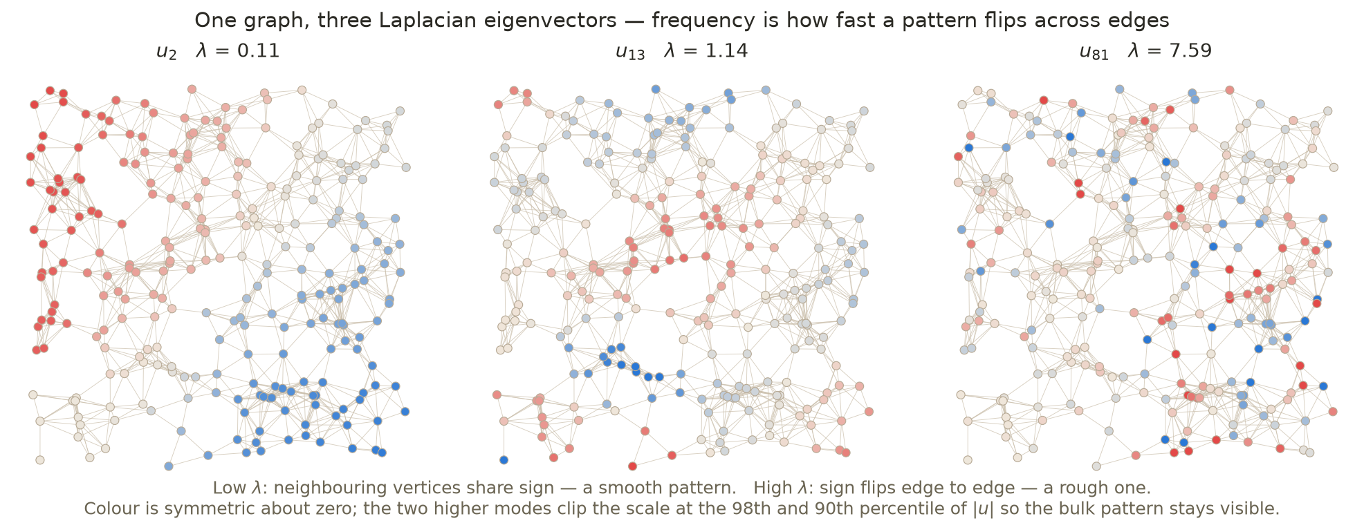
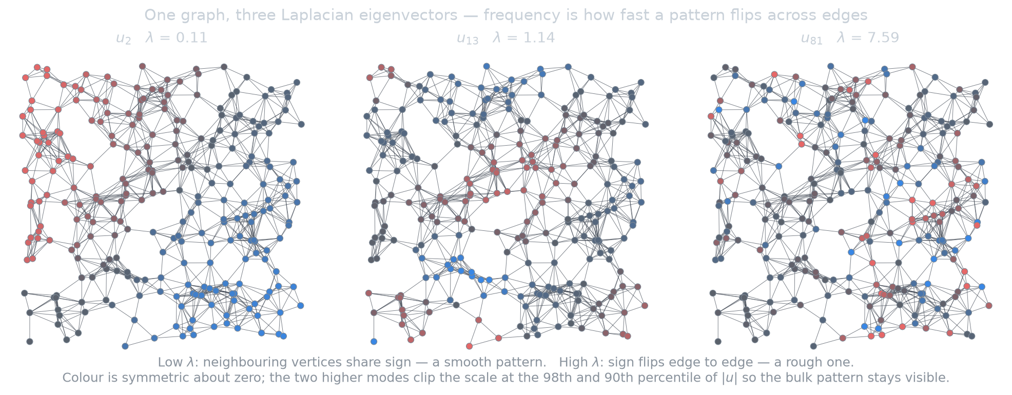
That is the whole intuition. There is no notion of “cycles per second” here, and no need for one. The ordering that matters is smooth to rough with respect to the graph, and the eigenvalue is the measure of roughness.
Once you have that ordering you have everything else by analogy. The graph Fourier transform of a signal \(x\) is its projection onto the eigenbasis, \(\hat{x} = U^\top x\). Filtering means reweighting those coefficients: keep the low ones and you have a low-pass filter, which on a graph means smoothing over the neighbourhood structure. Bandlimited means the signal is supported on the first few eigenvectors — and that is the assumption underpinning graph sampling theory, the same way bandlimitedness underpins Nyquist.
2013: the field gets a name, twice
Two papers appeared in 2013 that founded GSP, and they did not agree with each other.
Shuman, Narang, Frossard, Ortega, and Vandergheynst, “The Emerging Field of Signal Processing on Graphs” (IEEE Signal Processing Magazine, 2013), took the Laplacian as the fundamental operator, exactly as above. Frequency is variation; the graph Fourier transform is projection onto the Laplacian eigenbasis; low frequency means smooth across edges. This paper did the work of naming the field and mapping its open problems, and it is still the best single entry point.
Sandryhaila and Moura, “Discrete Signal Processing on Graphs” (IEEE Transactions on Signal Processing, 2013), took the adjacency matrix as the graph shift operator and rebuilt signal processing algebraically from it: filters as polynomials in the shift, convolution, z-transform, impulse and frequency response. Frequency comes from the eigendecomposition — or, when that fails, the Jordan decomposition — of A.
The disagreement is not cosmetic, and it is worth understanding because it still divides the literature.
| Laplacian route | Adjacency route | |
|---|---|---|
| Operator | L = D − A | A (the shift) |
| Frequency means | variation across edges | eigenvalue of the shift |
| Basis | real, orthogonal | generally neither |
| Directed graphs | not natively | yes |
| Recovers classical DSP | via the path graph | the cycle graph gives the DFT exactly |
| Natural home | smoothness, diffusion, clustering | filtering, algebraic theory |
The Laplacian route gives a real orthogonal eigenbasis and an intuitive smoothness ordering, but presumes an undirected graph. The adjacency route handles directed graphs and connects cleanly to classical DSP, but gives up orthogonality and a clean notion of “smooth.”
Both are still in use. Nearly all biological applications take the Laplacian route, and the reason is worth stating plainly: in biology the graph is usually a similarity or proximity graph, which is symmetric by construction, and “smooth over the graph” is exactly the hypothesis we want to test. We are rarely handed a directed graph we trust.
Consolidation (2014–2022)
The decade after 2013 rebuilt the standard toolkit roughly one classical concept at a time.
Sampling — which vertices must you measure to reconstruct a bandlimited graph signal — was worked out by Chen, Varma, Sandryhaila, and Kovačević (2015) and by Anis, Gadde, and Ortega (2016). The answers are less tidy than Nyquist: the optimal sampling set depends on the graph, and choosing it is combinatorial, so most of the work is on greedy and spectral-proxy approximations.
Filter banks and wavelets on graphs came largely from Narang and Ortega, who worked out critically sampled two-channel designs on bipartite graphs and the decomposition of arbitrary graphs into bipartite pieces.
Stationarity — the notion that a graph signal can be statistically shift-invariant, so that a power spectral density is meaningful — was defined independently by Perraudin and Vandergheynst and by Marques, Segarra, Leus, and Ribeiro. Without it there is no principled way to talk about noise on a graph.
Graph learning inverted the problem: given signals, infer the graph. Dong, Thanou, Frossard, and Vandergheynst approached it by assuming the observed signals are smooth on the unknown graph; Mateos, Segarra, Marques, and Ribeiro developed the network topology inference view. This matters in biology more than anywhere else, for a reason I return to at the end.
Vertex-frequency analysis — the graph analogue of a spectrogram, localising content in both vertex and frequency simultaneously — was developed by Shuman, Ricaud, and Vandergheynst. It reappears below in a place you might not expect.
The field acquired its textbook in 2022: Antonio Ortega’s Introduction to Graph Signal Processing (Cambridge). Tooling consolidated earlier around PyGSP, from Michaël Defferrard and Nathanaël Perraudin.
The fork that swallowed the field: graph neural networks
The largest branch of GSP is one most of its users do not call GSP.
Bruna, Zaremba, Szlam, and LeCun (2014) defined convolution on graphs spectrally — filters as multipliers in the Laplacian eigenbasis. This was elegant and impractical: it needs a full eigendecomposition, costs \(O(n^3)\), and the learned filters do not transfer between graphs.
Defferrard, Bresson, and Vandergheynst (2016) fixed it with ChebNet, approximating the spectral filter by a Chebyshev polynomial of L. A polynomial of degree K in L is K-hop local and needs no eigendecomposition at all — the filter is applied by repeated sparse matrix multiplication. Kipf and Welling (2017) truncated that polynomial to first order, renormalised, and produced the graph convolutional network that is now everywhere.
So a GCN layer is a first-order spectral graph filter with learned coefficients. Reading it that way is useful rather than pedantic. It explains oversmoothing directly: stacking layers means applying a low-pass filter repeatedly, and repeated low-pass filtering drives any signal toward the lowest frequency — the constant vector — so deep GCNs make every node representation converge to the same thing. It is also the basis for the stability and transferability theory of Gama, Bruna, and Ribeiro, and for the graphon signal processing that Ruiz, Chamon, and Ribeiro use to explain why a network trained on one graph works on a larger one drawn from the same generative model.
Where it went: sensors, brains, images, tissue
GSP spread first where the domain was irregular and physically real: sensor networks, transportation networks, point clouds and 3D meshes, and image and video coding, where Ortega’s group used graph transforms that adapt to edges a fixed DCT handles badly. Recommender systems were an early industrial adopter, since a user–item bipartite graph is the natural domain for ratings.
Biology arrived through two doors.
Door one: neuroimaging
The brain is the natural first case, because it comes with its graph already measured. Diffusion imaging supplies a structural connectome; functional imaging supplies a signal on it. You do not have to invent the domain.
Huang, Goldsberry, Wymbs, Grafton, Bassett, and Ribeiro, “Graph Frequency Analysis of Brain Signals” (IEEE JSTSP, 2016), decomposed brain activity into components aligned and misaligned with anatomy. Huang and colleagues extended this into a perspective piece in Proceedings of the IEEE (2018).
Preti and Van De Ville (Nature Communications, 2019) turned the idea into a measurement. Their structural decoupling index asks, per brain region, how much of the functional signal is smooth on the structural graph versus concentrated in high graph frequencies — that is, how much function follows structure. They find a macroscale gradient running from tightly coupled sensory regions to strongly decoupled higher-order association cortex.
This is the cleanest example I know of GSP producing a biological claim rather than a better filter. The result is not “we denoised the signal.” It is: the degree to which function follows structure is itself a regional property of the brain, it varies systematically, and the variation is behaviourally meaningful.
Door two: single-cell and spatial omics
The second door opens onto data with no given graph at all. In single-cell work we construct a cell–cell similarity graph — usually k nearest neighbours in some reduced expression space — and only then does the machinery apply.
The Krishnaswamy lab has been the most consistent force here, and the progression of their methods reads as a steady increase in how explicitly GSP is being used.
MAGIC (van Dijk et al., Cell, 2018) imputes dropout in scRNA-seq by diffusing expression over the cell–cell graph. In GSP terms it is a low-pass filter: powers of a Markov diffusion operator attenuate high graph frequencies, and dropout noise is high frequency because it is uncorrelated between neighbouring cells while real expression is not.
PHATE (Moon et al., Nature Biotechnology, 2019) uses diffusion geometry for visualisation that preserves trajectory structure rather than only local neighbourhoods.
MELD (Burkhardt et al., Nature Biotechnology, 2021) is the most explicitly GSP of the three. It treats the experimental label — treated or control — as a signal on the cell graph, low-pass filters it to get a smooth estimate of how enriched each region of the manifold is for the perturbation, and then applies vertex-frequency clustering — Shuman’s construction, arriving in cell biology a decade after it was designed for signal processing — to find cell populations that respond uniformly. That is a full round trip: a tool built for localisation on graphs, used to answer “which cells actually responded to the drug.”
More recently, gene signal pattern analysis learns gene representations from a dictionary of diffusion wavelets on the cell–cell graph, moving the object of study from cells-as-vertices to genes-as-signals.
Spatial omics is the newest case and, to my mind, the most natural one — because the graph is not inferred from similarity at all. It is given by physical adjacency in tissue. Two spots are neighbours if they are next to each other, which is a fact about the specimen rather than a modelling choice about expression space.
Once the graph is physical, a gene’s expression across spots is a signal on it, and the graph Fourier transform does something immediately useful:
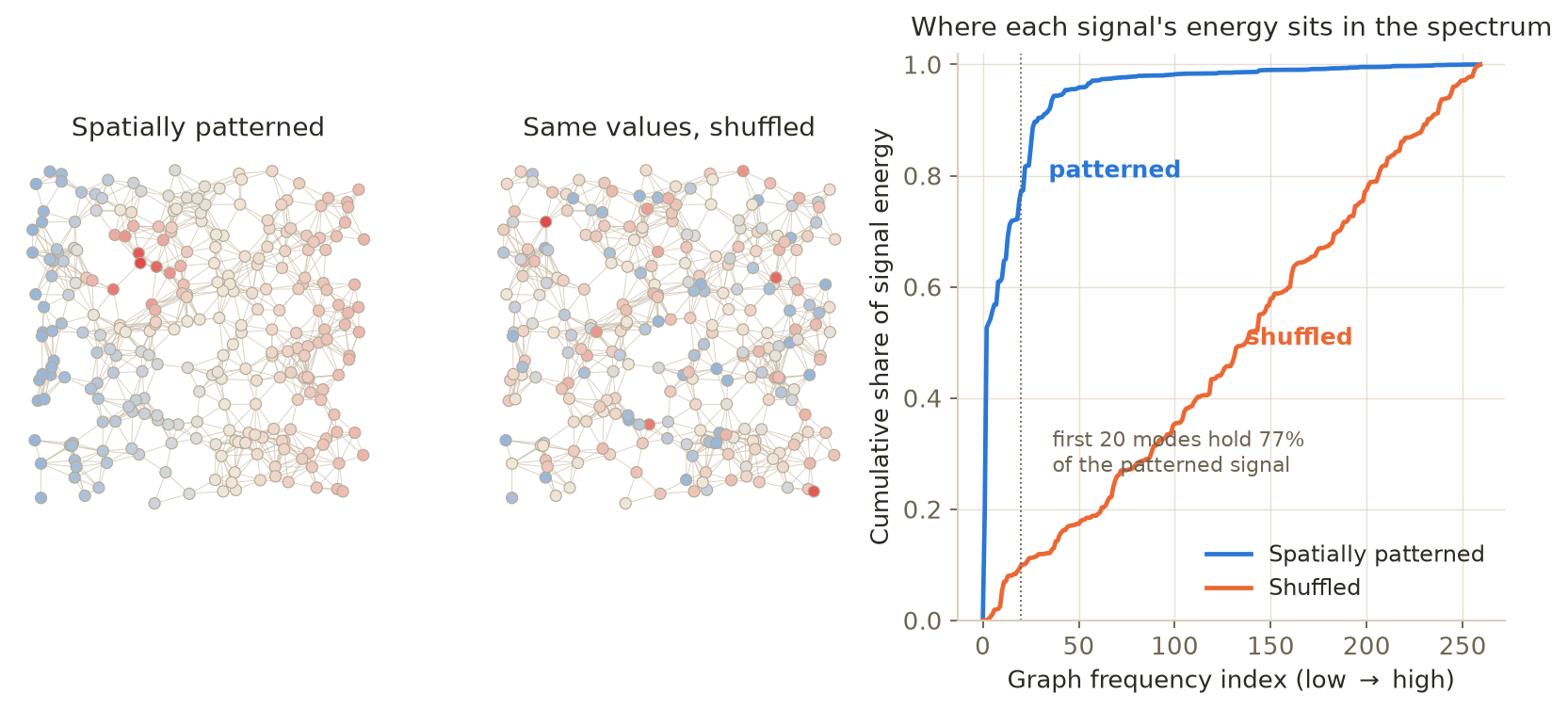
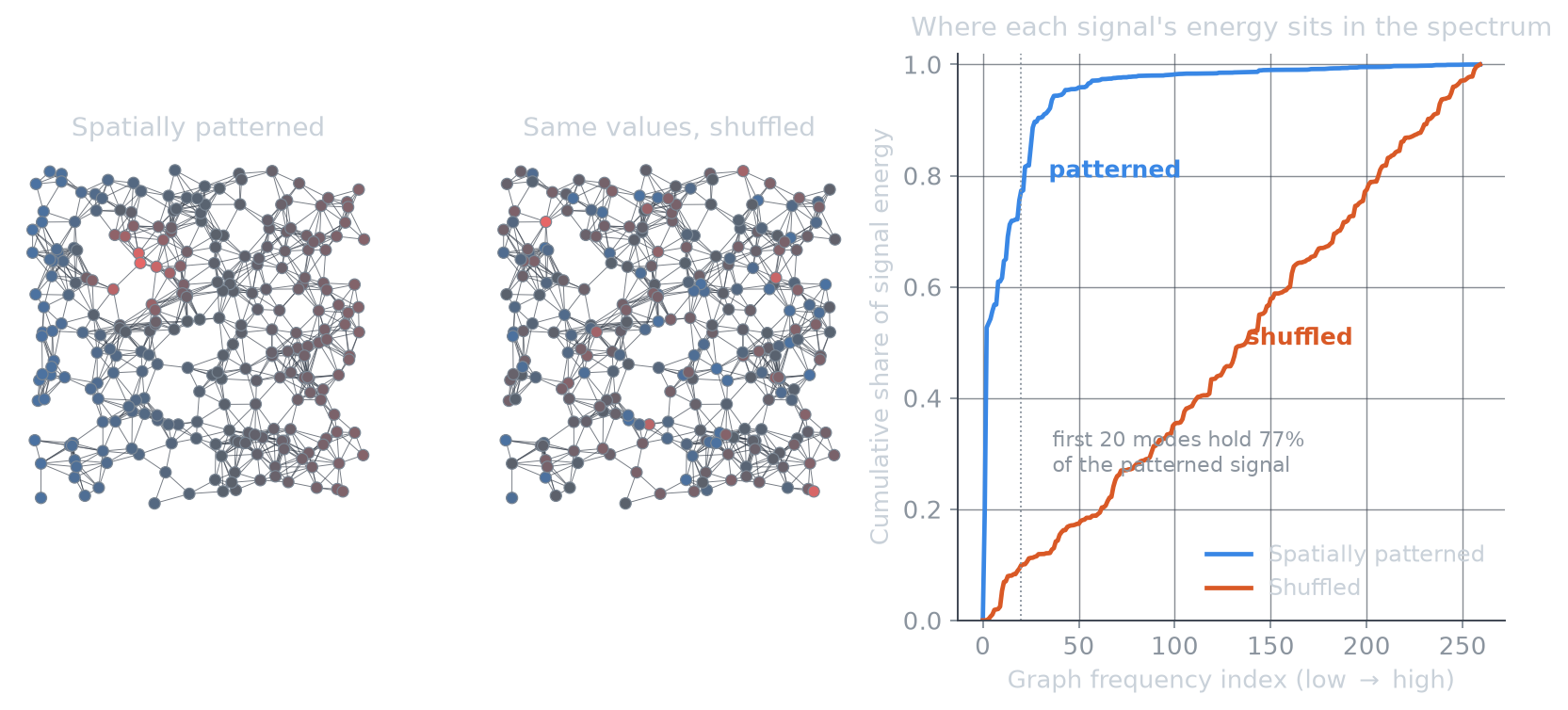
The point of that figure is the identical marginal distribution. Spatial pattern is not a property of the values a gene takes; it is a property of how those values sit on the graph. The graph Fourier transform is a direct measurement of exactly that, so detecting a spatially variable gene becomes a question about where its energy lies in the spectrum rather than a per-gene statistical test with a spatial covariance model bolted on. Grouping genes by their spectral profile then yields multicellular regions that may overlap, rather than a hard partition of the tissue into domains.
(This is the line my own work sits on — SpaGFT, Chang et al., Nature Communications 15:7467, 2024 — so read this section as an interested party’s account of it.)
Who is building it now
An incomplete list, grouped by contribution. Corrections are welcome; any field map drawn by one person reflects where that person is standing.
Foundations and theory. Antonio Ortega (USC) — sampling, graph learning, image coding, and the field’s textbook. Pierre Vandergheynst and Pascal Frossard (EPFL) — spectral graph wavelets, stationarity, and much of the original framing. José M. F. Moura (CMU) and Jelena Kovačević (NYU) — the algebraic, adjacency-based formulation and sampling theory. David Shuman (Olin) — vertex-frequency analysis and the 2013 synthesis.
Networks, inference, and statistics. Alejandro Ribeiro (Penn) — graph neural network theory, stability, graphon signal processing. Antonio G. Marques (URJC), Santiago Segarra (Rice), Gonzalo Mateos (Rochester), and Geert Leus (TU Delft) — stationarity, topology inference, and the statistical foundations. Xiaowen Dong (Oxford) — learning graphs from data.
The deep-learning bridge. Michaël Defferrard — ChebNet and PyGSP. Michael Bronstein (Oxford) — geometric deep learning, which places GSP inside a broader program about symmetry and structure in learning.
Neuroscience. Dimitri Van De Ville (EPFL / Geneva) — structure–function coupling and the decoupling index. Danielle Bassett (Penn) — network neuroscience. Selin Aviyente (Michigan State) — graph and time-vertex methods for neurophysiological signals.
Biology and single-cell. Smita Krishnaswamy (Yale) and Guy Wolf (Université de Montréal / Mila) — diffusion geometry and the line running from MAGIC and PHATE through MELD to gene-level signal analysis. Their body of work is the main reason GSP has a foothold in molecular biology at all.
What is still open
Three problems seem to me to matter most, and the third is the one biology forces.
Directed graphs. Gene regulation, signalling cascades, and information flow are directed, but the Laplacian machinery assumes symmetry, and the adjacency formulation buys direction at the cost of an orthogonal basis and a clean smoothness ordering. Various magnetic and Hermitian Laplacians exist; none has become standard. For a field whose most important biological objects are directed, this is a real gap.
Dynamic and higher-order structure. Tissue changes, connectomes reconfigure, and many biological interactions are not pairwise — a protein complex is not a set of edges. Time-varying graph signal processing and the simplicial and hypergraph extensions are active areas, and neither is settled.
The graph is a modelling choice, not data. This is the one I would put effort into. In neuroimaging the connectome is measured. In single-cell and spatial omics we construct the graph — k nearest neighbours, a distance threshold, a kernel bandwidth — and every spectral quantity downstream inherits that choice. Change k and the Laplacian changes, so the eigenvectors change, so the frequency ordering changes, so which genes look “spatially variable” changes.
The field has good theory for inferring a graph from signals. What it has much less of is practice for reporting how much a biological conclusion depends on the graph it was computed on. A spatially variable gene detected at k = 6 and absent at k = 10 is not a finding, but nothing in the standard workflow forces that check. Sensitivity to graph construction should be reported the way we report sensitivity to a clustering resolution — and mostly it is not.
Corrections and additions are welcome, particularly for work I have under-represented. The history above is compressed, and the boundary between “graph signal processing” and its neighbours in spectral clustering, manifold learning, and geometric deep learning is a matter of convention rather than fact.